Stream Evaluators
To estimate prediction measures in the context of data streams with
strict computational requirements and concept drifts, the evaluators module
of the stream-learn package implements two main estimation techniques
described in the literature in their batch-based versions.
Test-Then-Train Evaluator
The TestThenTrain class implements the Test-Then-Train evaluation procedure,
in which each individual data chunk is first used to test the classifier before
it is used for updating the existing model.

The performance metrics returned by the evaluator are determined by the
metrics parameter which accepts a tuple containing the functions of preferred quality
measures and can be specified during initialization.
Processing of the data stream is started by calling the process() function
which accepts two parameters (i.e. stream and clfs) responsible for
defining the data stream and classifier, or a tuple of classifiers, employing
the partial_fit() function. The size of each data chunk is determined by
the chunk_size parameter from the StreamGenerator class. The results
of evaluation can be accessed using the scores attribute, which is a
three-dimensional array of shape (n_classifiers, n_chunks, n_metrics).
Example – single classifier
from strlearn.evaluators import TestThenTrain
from strlearn.ensembles import SEA
from strlearn.utils.metrics import bac, f_score
from strlearn.streams import StreamGenerator
from sklearn.naive_bayes import GaussianNB

stream = StreamGenerator(chunk_size=200, n_chunks=250)
clf = SEA(base_estimator=GaussianNB())
evaluator = TestThenTrain(metrics=(bac, f_score))

evaluator.process(stream, clf)
print(evaluator.scores)
Example – multiple classifiers
from strlearn.evaluators import TestThenTrain
from strlearn.ensembles import SEA
from strlearn.utils.metrics import bac, f_score
from strlearn.streams import StreamGenerator
from sklearn.naive_bayes import GaussianNB
from sklearn.tree import DecisionTreeClassifier

stream = StreamGenerator(chunk_size=200, n_chunks=250)
clf1 = SEA(base_estimator=GaussianNB())
clf2 = SEA(base_estimator=DecisionTreeClassifier())
clfs = (clf1, clf2)
evaluator = TestThenTrain(metrics=(bac, f_score))

evaluator.process(stream, clfs)
print(evaluator.scores)
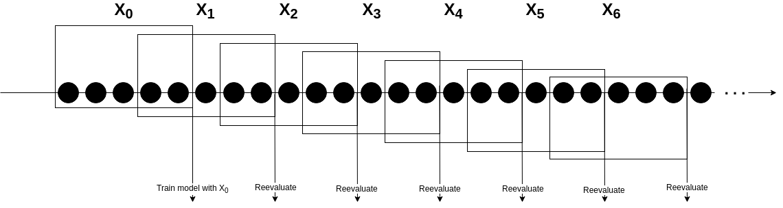
Prequential Evaluator
The Prequential procedure of assessing the predictive performance of stream
learning algorithms is implemented by the Prequential class. This estimation
technique is based on a forgetting mechanism in the form of a sliding window
instead of a separate data chunks. Window moves by a fixed number of instances
determined by the interval parameter for the process() function. After each
step, samples that are currently in the window are used to test the classifier
and then for updating the model.
Similar to the TestThenTrain evaluator, the object of the Prequential
class can be initialized with a metrics parameter containing metrics names
and the size of the sliding window is equal to the chunk_size parameter from
the instance of StreamGenerator class.
Example – single classifer
from strlearn.evaluators import Prequential
from strlearn.ensembles import SEA
from strlearn.utils.metrics import bac, f_score
from strlearn.streams import StreamGenerator
from sklearn.naive_bayes import GaussianNB

stream = StreamGenerator()
clf = SEA(base_estimator=GaussianNB())
evaluator = TestThenTrain(metrics=(bac, f_score))

evaluator.process(stream, clf, interval=100)
print(evaluator.scores)
Example – multiple classifiers
from strlearn.evaluators import Prequential
from strlearn.ensembles import SEA
from strlearn.utils.metrics import bac, f_score
from strlearn.streams import StreamGenerator
from sklearn.naive_bayes import GaussianNB
from sklearn.tree import DecisionTreeClassifier

stream = StreamGenerator(chunk_size=200, n_chunks=250)
clf1 = SEA(base_estimator=GaussianNB())
clf2 = SEA(base_estimator=DecisionTreeClassifier())
clfs = (clf1, clf2)
evaluator = Prequential(metrics=(bac, f_score))

evaluator.process(stream, clfs, interval=100)
print(evaluator.scores)
Metrics
To improve the computational performance of presented evaluators, the
stream-learn package uses its own implementations of metrics for classification
of imbalanced binary problems, which can be found in the utils.metrics module.
All implemented metrics are based on the confusion matrix.

Recall
Recall (also known as sensitivity or true positive rate) represents the classifier’s ability to find all the positive data samples in the dataset (e.g. the minority class instances) and is denoted as
Example
from strlearn.utils.metrics import recall
Precision
Precision (also called positive predictive value) expresses the probability of correct detection of positive samples and is denoted as
Example
from strlearn.utils.metrics import precision
F-beta score
The F-beta score can be interpreted as a weighted harmonic mean of precision and
recall taking both metrics into account and punishing extreme values. The beta parameter determines the recall’s weight. beta < 1 gives more weight to precision, while beta > 1 prefers recall.
The formula for the F-beta score is
Example
from strlearn.utils.metrics import fbeta_score
F1 score
The F1 score can be interpreted as a F-beta score, where \(\beta\) parameter equals 1. It is a harmonic mean of precision and recall. The formula for the F1 score is
Example
from strlearn.utils.metrics import f1_score
Balanced accuracy (BAC)
The balanced accuracy for the multiclass problems is defined as the average of recall obtained on each class. For binary problems it is denoted by the average of recall and specificity (also called true negative rate).
Example
from strlearn.utils.metrics import bac
Geometric mean score 1 (G-mean1)
The geometric mean (G-mean) tries to maximize the accuracy on each of the classes while keeping these accuracies balanced. For N-class problems it is a N root of the product of class-wise recall. For binary classification G-mean is denoted as the squared root of the product of the recall and specificity.
Example
from strlearn.utils.metrics import geometric_mean_score_1
Geometric mean score 2 (G-mean2)
The alternative definition of G-mean measure. For binary classification G-mean is denoted as the squared root of the product of the recall and precision.
Example
from strlearn.utils.metrics import geometric_mean_score_2
References
Ricardo A. Baeza-Yates and Berthier Ribeiro-Neto. Modern Information Retrieval. Addison-Wesley Longman Publishing Co., Inc., Boston, MA, USA, 1999. ISBN 020139829X.
Ricardo Barandela, Josep Sánchez, Vicente García, and E. Rangel. Strategies for learning in class imbalance problems. Pattern Recognition, 36:849–851, 03 2003.
Kay Henning Brodersen, Cheng Soon Ong, Klaas Enno Stephan, and Joachim M. Buhmann. The balanced accuracy and its posterior distribution. In Proceedings of the 2010 20th International Conference on Pattern Recognition, ICPR '10, 3121–3124. Washington, DC, USA, 2010. IEEE Computer Society.
Joao Gama. Knowledge Discovery from Data Streams. Chapman & Hall/CRC, 1st edition, 2010. ISBN 1439826110, 9781439826119.
João Gama, Raquel Sebastião, and Pedro Pereira Rodrigues. On evaluating stream learning algorithms. Machine Learning, 90(3):317–346, Mar 2013.
John D. Kelleher, Brian Mac Namee, and Aoife D'Arcy. Fundamentals of Machine Learning for Predictive Data Analytics: Algorithms, Worked Examples, and Case Studies. The MIT Press, 2015. ISBN 0262029448, 9780262029445.
Miroslav Kubat and Stan Matwin. Addressing the curse of imbalanced training sets: one-sided selection. In ICML. 1997.
David Powers and Ailab. Evaluation: from precision, recall and f-measure to roc, informedness, markedness & correlation. J. Mach. Learn. Technol, 2:2229–3981, 01 2011.
Yutaka Sasaki. The truth of the f-measure. Teach Tutor Mater, pages, 01 2007.